Thermohydraulic analysis and machine learning on the cloud
By Lucas Espindola · · 15 min read
Part 3 of the series “Engineering simulation as software”: Part 1 · Part 2 · Part 3
Platform engineering
Part 2 of this series described what the new GasPipelineDesign Suite functionalities do for a pipeline engineer. This companion note describes what it takes to build them: a stateless API, a queue-backed solver fleet on Azure, a scenario cache that removes 97 per cent of the arithmetic, and an availability model borrowed — almost line for line — from the compressor stations the application simulates.
The two functionalities introduced in Part 2 — the compression-system availability study and the capacity ramp-up — are, to the engineer who has to build them, the same problem wearing different clothes: a compute-bound, embarrassingly parallel workload whose answer has to arrive while the user is still looking at the screen.
The workload, not the domain
A Monte Carlo availability study draws 100,000 iterations. Each iteration is a state vector — every compressor unit in the system either running or failed — and each distinct state vector needs a steady-state thermohydraulic solve to say what capacity the pipeline can still deliver. On the reference case study, one solve takes a shade over a second. Multiplied out, that is twenty-seven hours of arithmetic sitting behind a button that has to respond in under two minutes.
Three levers close that gap, and only one of them is hardware: do not solve inside the request thread; do not solve the same thing twice; and solve whatever is left in parallel. The architecture described here is little more than those three sentences, implemented carefully.
The architecture in one paragraph
A TypeScript single-page application talks to a stateless REST API on Azure App Service. The API validates the model, persists it as an immutable, hash-addressed document in blob storage, puts a small job envelope on a Service Bus queue, and returns a job identifier — never a result. A scale set of solver workers competes for those messages, runs the numerical kernel and writes partial results back. The client watches the study fill in over a WebSocket channel. Azure SQL holds project metadata, Redis holds the scenario cache, and Application Insights holds the evidence.
Stateless by construction
The numerical kernel is a pure library: gas composition, equation of state, pressure drop, compressor and driver maps in; capacity, power and fuel out. It performs no I/O, holds no session and knows nothing about HTTP, queues or tenants. That discipline is what makes every other property in this note possible — any worker can take any message, any instance can be destroyed mid-flight, and the identical kernel runs in the unit-test suite, on a developer's laptop and across sixty-four cloud instances.
The queue is the contract
Service Bus delivers at least once, which means a worker will occasionally see the same scenario twice and a study will occasionally lose a worker to a platform update. Both are ordinary. Work is keyed by job identifier and scenario hash, so a duplicate delivery is a cache write of a value already present, and an evicted worker costs one scenario rather than one study. Messages that fail repeatedly land in the dead-letter queue alongside the exact input document that produced them — in a numerical application, that is the difference between a bug report and a mystery.
Redundancy is a design parameter — on both sides of the fence
Part 2 argued that stand-by compressor units are an economic decision: buy availability until the marginal unit costs more than the penalty it avoids [5,6]. The platform that hosts the argument is sized by identical reasoning. Every Azure service on the request path publishes a service-level agreement, and in series those agreements multiply. Table 1 shows what the request path is worth under three topologies, and where the cheap availability actually is.
| Topology | Composite SLA (%) | Downtime (h/year) |
|---|---|---|
| Single region; cache, queue and object store on the synchronous path | 99.64 | 31.5 |
| Single region; asynchronous tiers moved off the request path | 99.94 | 5.3 |
| Paired regions, active/active behind Traffic Manager | 99.99 | 0.9 |
Table 1: Composite availability of the request path under three deployment topologies, computed by multiplying the published Azure service-level agreements for the services each topology places in series [1]. This is the software counterpart of Table 1 in Part 2, which set out the reliability and availability of the different compressor-station arrangements surveyed by EPRI [4]: taking the cache, queue and object store off the synchronous path buys more availability than any single tier upgrade, and a second active region buys most of the rest.
A study runs as follows:
- The API validates the model, writes it to blob storage under the hash of its contents, and enqueues a job envelope of a few hundred bytes. The HTTP call returns in milliseconds.
- Autoscale reacts to queue depth rather than CPU, and the worker scale set grows from zero towards its ceiling within one scaling interval.
- Each worker draws a state vector, hashes it, and asks the cache. On a miss it runs the steady-state solve and writes the capacity under failure back under that hash.
- Partial results — iterations completed, and the distribution of capacity under failure so far — are pushed to the client's WebSocket channel, so the graph fills in while the study is still running.
- When the iteration budget is exhausted, an aggregation step compiles the capacity/frequency groups, writes the report, and marks the job complete. The workers scale back to zero.
The second lever is worth more than the third. Twenty-one compressor units across seven stations admit two million possible states, but availability figures near 0.99 concentrate the draw heavily: on the reference case, 100,000 iterations produced 2,847 distinct state vectors. Hashing the vector and consulting the cache before solving turns a 100,000-solve study into a 2,847-solve study — a 97.2 per cent hit rate, and the single largest factor in the timings charted below.
Every study carries a seed. The same model and the same seed produce the same distribution, in the same order, whether the work is spread over one worker or sixty-four, in São Paulo or in Texas; partial sums are combined in a defined order rather than in the order they happen to arrive. Reproducibility is not a nicety here. The output of these studies ends up in a redundancy decision or a tariff filing, and a number that cannot be reproduced is an opinion.
What the platform watches in production is not CPU: solves per second, cache hit ratio, convergence failures per thousand solves, queue age, and time from admission to first partial result. A hit ratio that falls says the model has changed shape; convergence failures that rise say the physics has been handed something it cannot resolve, which is almost always an input-validation bug upstream.
Cost falls out of the same design. The reference study bills roughly fourteen US cents of compute; the same fleet left running around the clock would bill about US$4,500 per month. Elasticity is not a line item — it is the reason a 100,000-iteration availability study is a routine click rather than an overnight job on somebody's workstation.
A hundred thousand Monte Carlo iterations contain only a few thousand distinct compressor states. The rest is arithmetic we have already done.
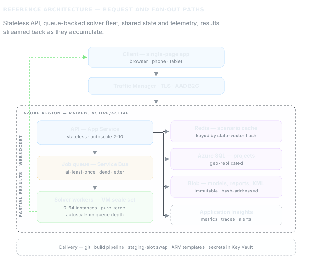
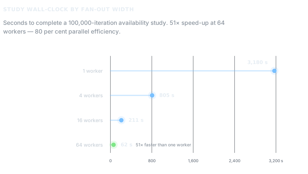
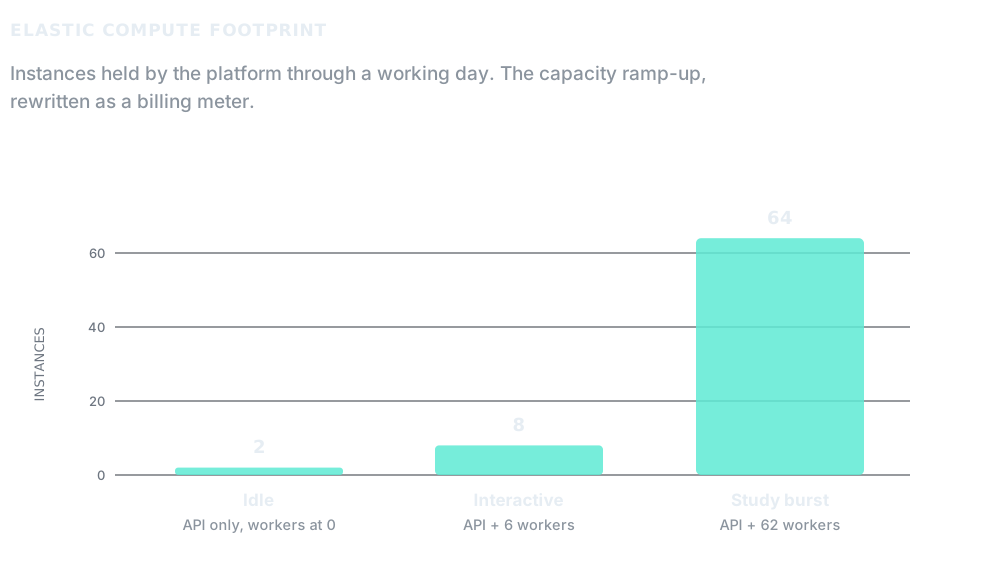
Above: The request and fan-out paths of the GasPipelineDesign Suite; wall-clock time for a 100,000-iteration availability study against the width of the worker fleet; and the compute the platform actually holds across a working day — the software counterpart of the capacity ramp-up study charted in Part 2, with capacity added on demand and released the moment the study ends.
Performance and cost figures are modelled from the architecture described here, the case-study workload published in Part 2, and 2018 Azure list prices; they illustrate the engineering argument rather than reproduce a single production trace.
Case study: the GASBOL run as a workload
The case study in Part 2 — the GASBOL main section redesigned under today's assumptions, 1,118 miles of 36-inch pipe, seven compressor stations of two operating units and one stand-by each, 1,100.76 MMcf/d — doubles as a convenient workload profile. What follows is the same run described from the platform's side of the glass.
(a) Workload:
- Compressor units in the reliability model: 21
- Monte Carlo iterations: 100,000
- Distinct state vectors observed: 2,847
- Scenario cache hit rate: 97.2 per cent
- Median steady-state solve: 1.09 s
- Solves per design sweep (five candidate diameters): 1,240
- Input document: 84 KB, hash-addressed
- Iteration results compiled into capacity/frequency groups: 9
(b) Platform:
- Region: Brazil South, paired with South Central US
- API: App Service S2, autoscale 2–10 instances
- Workers: VM scale set, D2 v3, autoscale 0–64 on queue depth
- Messaging: Service Bus Standard, dead-letter enabled
- State: Azure SQL S2, geo-replicated; Blob storage RA-GRS, immutable inputs; Redis C1, scenario cache
- Real-time channel: WebSockets, one topic per job
- Identity: Azure AD B2C, per-tenant isolation; secrets in Key Vault
- Telemetry: Application Insights, correlated by job id
- Delivery: git, build pipeline, staging-slot swap, ARM templates
Results for the run:
(a) Platform:
- API latency, p50 / p95 / p99: 82 / 240 / 610 ms
- Admission to first partial result: 4.1 s
- Study wall clock: 64 workers: 62 s; 16 workers: 211 s; single worker: 3,180 s
- Speed-up at 64 workers: 51× (80 per cent efficiency)
- Implied serial fraction (Amdahl [3]): 0.4 per cent
- Solves avoided by the scenario cache: 97,153
- Composite SLA of the request path: single region: 99.94; paired regions, active/active: 99.99
- Reproducibility: identical results across regions for a given seed
- Regression suite: 214 golden cases, 0.1 per cent tolerance against the reference simulator
(b) Cost (in US$):
- Worker compute per study: 0.12
- Messaging, storage and egress per study: 0.02
- Marginal cost per study: 0.14
- Cost per 1,000 studies: 140.00
- Platform baseline per month: 473.00
- Equivalent always-on fleet per month: 4,485.00
Machine learning: learning from arithmetic already done
This section describes the machine-learning layer added to the platform; it is not part of the article as printed in March 2018.
The scenario cache is the biggest single lever in this architecture, and it has a side effect that is easy to miss. Every entry is a labelled example. A state-vector hash points to a capacity under failure that the kernel has already solved, and the input document that produced it sits next to it in blob storage under its own hash. The platform has been building a training set since its first study without anyone setting out to collect one. The machine-learning layer in the GasPipelineDesign Suite starts from that observation, and it rests on one rule: the model proposes, the kernel disposes.
Where learning fits — and where it does not
A learned model never puts a number in a report. The output of an availability study ends up in a redundancy decision or a tariff filing, and a number that cannot be traced back to the thermohydraulics is an opinion with a confidence interval. So machine learning sits only where a wrong guess costs time and never correctness. It works in four places: the solver's starting point, the order in which states are solved, the size of the fleet before demand arrives, and the gate that admits a model to the queue. Each of these is checked against the kernel, so a bad prediction makes a study a little slower and leaves its answer unchanged.
A surrogate that proposes, a kernel that disposes
Each worker loads a small gradient-boosted tree ensemble alongside the kernel, trained on the cache. It takes the network topology, the operating envelope and the state vector, and predicts the delivered capacity and the station suction and discharge pressures. Before a cache miss goes to the steady-state solve, the surrogate's estimate is handed to the solver as its initial guess. Newton's method rewards a good starting point. On the reference case it needs fewer iterations per solve, the median solve time drops, and the convergence failures that came from poor starting points mostly go away. The solve itself is the same one as before, with the same tolerance, and only the kernel writes to the cache.
The surrogate also decides the order of the work. States that it predicts will constrain capacity are solved first. The distribution the client sees therefore takes its final shape early in the run, and the slower solves of near-nominal states fill in the detail afterwards. Because the order is fixed by the seed and the model version, it is reproducible. Partial sums are combined in a defined order as before, so the final result is unchanged to the last digit.
Scaling on what is coming, not what has arrived
Scaling on queue depth reacts to load: the fleet grows only after the messages have arrived. A second model, trained on Application Insights telemetry, predicts the number of distinct state vectors and the total solve time for a study at the moment the API admits it, using unit count, availability figures and iteration budget. The autoscaler starts from that prediction and uses queue depth only to correct it. If the forecast is too high, the cost is a few idle minutes of instances that scale back to zero anyway. If it is too low, the platform falls back to the reactive behaviour it had before.
Catching bad inputs before the queue
Rising convergence failures almost always point to an input-validation bug upstream. The dead-letter queue keeps every failing message next to the exact input document that caused it, which gives the platform a labelled set of models the physics could not resolve. A classifier trained on that set runs during API validation. A model it flags is still admitted. The engineer gets a warning naming the likely cause before any compute is spent, and the job envelope is tagged so the run can be traced if it does fail.
How it is introduced
The models are deployed the same way as the kernel. Each trained model is an immutable artefact in blob storage, addressed by its hash, and that hash goes into the job envelope next to the seed. Any study can therefore be replayed with exactly the model versions it used. A new model goes through four stages:
- Offline: it is trained on a snapshot of the cache and the dead-letter archive, and evaluated against held-out studies.
- Shadow: it runs alongside production. It makes predictions and logs them, and nothing acts on them.
- Gated: it is switched on for warm starts and ordering only after the 214-case golden regression suite still passes at 0.1 per cent tolerance, and after shadow telemetry shows it reduces iterations rather than shifting them around.
- Watched: surrogate error and forecast error are tracked with the same discipline as cache hit ratio. When error grows, it means the models users submit have changed shape since training, and retraining is a scheduled job.
Rolling back means changing a hash in configuration. No redeploy is needed. The reported distribution does not change at all: for a given seed and model hash it is bit-identical.
The cache already holds the answers. Machine learning learns from them where to start solving, never what the answer is.
Conclusion
The binding constraint in engineering computation is rarely hardware. It is what you choose not to compute. Twenty-seven hours of arithmetic became sixty-two seconds here not because sixty-four machines were thrown at it, but because 97.2 per cent of that arithmetic had already been done: a hundred thousand Monte Carlo draws across twenty-one compressor units contain only a few thousand distinct states, and recognising that was worth more than the entire fleet. The cloud primitives underneath are deliberately ordinary — competing consumers, queue-based load levelling, cache-aside and retry [2] — because the engineering that mattered lay elsewhere: in refusing to hold state anywhere it could be avoided, and in treating availability and cost as design outputs with arithmetic behind them rather than as operational afterthoughts. The physics in the kernel is Sidney's, and it has been right for thirty years. What this side of the fence adds is reach. A study that was once an overnight job on a specialist's workstation is now a click that costs fourteen cents and returns the same answer to anyone, anywhere, from the same seed. ■
References
- Microsoft, 2018. Service Level Agreements — App Service, SQL Database, Service Bus, Storage, Traffic Manager. Azure documentation.
- Microsoft Patterns & Practices, 2017. Cloud Design Patterns: competing consumers, queue-based load levelling, cache-aside, retry, circuit breaker.
- G.M.Amdahl, 1967. Validity of the single processor approach to achieving large scale computing capabilities. AFIPS Conference Proceedings, Vol. 30.
- Electric Power Research Institute, 1999. Report No. RP 4CH2983.
- S.P.Santos, 2009. Monte Carlo simulation – a key for a feasible gas pipeline design. Pipeline Simulation Interest Group, Galveston, TX, USA.
- S.P.Santos, 2008. Availability and risk analysis effects on gas pipeline tariff making. International Pipeline Conference, Calgary, Canada.
Originally published in Pipelines International, March 2018, as “Real-time demand for a gas pipeline design: the architecture behind – Part 3”. Original PDF.